标签传播算法

LPA算法简介

标签传播算法（Label Propagation Algorithm，LPA）是由Zhu等人于2002年提出，它是一种基于图的半监督学习方法，其基本思路是用已标记节点的标签信息去预测未标记节点的标签信息。

​ LPA算法思路简单清晰，其基本过程如下：

1. 为每个节点随机的指定一个自己特有的标签；
2. 逐轮刷新所有节点的标签，直到所有节点的标签不再发生变化为止。对于每一轮刷新，节点标签的刷新规则如下：

​ 对于某一个节点，考察其所有邻居节点的标签，并进行统计，将出现个数最多的那个标签赋值给当前节点。当个数最多的标签不唯一时，随机选择一个标签赋值给当前节点。

在标签传播算法中，节点的标签更新通常有同步更新和异步更新两种方法。同步更新是指，节点x在t时刻的更新是基于邻接节点在t-1时刻的标签。异步更新是指，节点x在t时刻更新时，其部分邻接节点是t时刻更新的标签，还有部分的邻接节点是t-1时刻更新的标签。LPA算法在标签传播过程中采用的是同步更新，研究者们发现同步更新应用在二分结构网络中，容易出现标签震荡的现象。因此，之后的研究者大多采用异步更新策略来避免这种现象的出现。

LPA算法

相似矩阵构建

令( x1，y1) …( xl，yl) 是已标注数据，YL={ y1…yl} ∈{ 1…C} 是类别标签，类别数 C 已知，且均存在于标签数据中。令( xl + 1，yl + 1) …( xl + u，yl + u) 为未标注数据，YU={ yl + 1…yl + u} 不可观测，l << u，n=l+u。令数据集 X = { x1…xl + u} ∈R。问题转换为: 从数据集 X 中，利用YL的学习，为未标注数据集YU的每个数据找到对应的标签。将所有数据作为节点( 包括已标注和未标注数据) ，创建一个图，这个图的构建方法有很多，这里我们假设这个图是全连接的，节点i和节点j的边权重为：

$\large w_{ij}=exp(-\frac{||x_i-x_j||^2}{\alpha^2})$

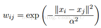
这里，α是超参。还有个非常常用的图构建方法是knn图，也就是只保留每个节点的k近邻权重，其他的为0，也就是不存在边，因此是稀疏的相似矩阵。

LPA算法

标签传播算法非常简单：通过节点之间的边传播label。边的权重越大，表示两个节点越相似，那么label越容易传播过去。我们定义一个NxN的概率转移矩阵P：

$\Large P_{ij}=P(i\to j)=\frac{w_{ij}}{\sum_{k=1}^{n}w_{ik}}$

​ Pij表示从节点i转移到节点j的概率。我们将YL和YU合并，我们得到一个NxC的soft label矩阵F=[YL;YU]。soft label的意思是，我们保留样本i属于每个类别的概率，而不是互斥性的，这个样本以概率1只属于一个类。当然了，最后确定这个样本i的类别的时候，是取max也就是概率最大的那个类作为它的类别的。那F里面有个YU，它一开始是不知道的，那最开始的值是多少？无所谓，随便设置一个值就可以了。

​ 简单的LP算法如下：

1. 执行传播：F=PF；
2. 重置F中labeled样本的标签：FL=YL；
3. 重复步骤（1）和（2）直到F收敛。

​ 步骤（1）就是将矩阵P和矩阵F相乘，这一步，每个节点都将自己的label以P确定的概率传播给其他节点。如果两个节点越相似（在欧式空间中距离越近），那么对方的label就越容易被自己的label赋予。步骤（2）非常关键，因为labeled数据的label是事先确定的，它不能被带跑，所以每次传播完，它都得回归它本来的label。

变身的LPA算法

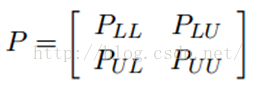
我们知道，我们每次迭代都是计算一个soft label矩阵F=[YL;YU]，但是YL是已知的，计算它没有什么用，在步骤（2）的时候，还得把它弄回来。我们关心的只是YU，那我们能不能只计算YU呢？我们将矩阵P做以下划分：

令 ，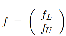

这时候，我们的算法就一个运算：

​ 迭代上面这个步骤直到收敛就ok了。可以看到fU不但取决于labeled数据的标签及其转移概率，还取决了unlabeled数据的当前label和转移概率。因此LP算法能额外运用unlabeled数据的分布特点。

收敛性证明

当n趋近于无穷大是，有

$\large f_U= \lim\limits_{n\to\infty} (P_{UU})^nf_U^0+(\sum_{i=1}^n(P_{UU}^{i-1})P_{UL}Y_L$

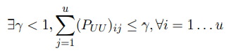
其中$f_U^0$是fU的初始值，因此我们需要证明 因为P是行标准化的，并且PUU是P的子矩阵，所以

，

因此

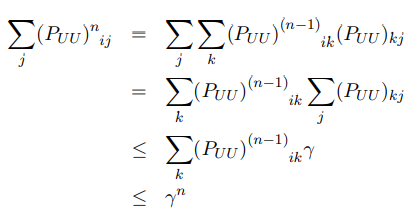
当n趋近于无穷大时，rn=0，（PUU)n收敛于0，也意味着因此的初始值是无关紧要的，同时第n次迭代时fU收敛。

标签传播算法的基本特点

(1) LPA是一种半监督学习方法，具有半监督学习算法的两个假设前提：1. 临近样本点具有相同的标签。根据该假设，分类时边界两侧尽可能避免选择较为密集的样本数据点，而是尽量选择稀疏数据，便于算法利用少了已标注数据指导大量的未标注数据。2. 相同流结构上的点能够拥有相同的标签。根据该假设，未标记的样本数据能够让数据空间变得更加密集，便于充分分析局部区域特征。
(2) LPA只需要利用少量的训练标签指导，利用未标注数据的内在结构，分布规律和临近数据的标记，即可预测和传播未标记数据的标签，然后合并到标记的数据集中。该算法操作简单，运算量小，适合大规模数据信息的挖掘和处理。
(3) LPA 可以通过相近节点之间的标签的传递来学习分类，所以它不受数据分布形状的局限。所以只要同一类的数据在空间分布上是相似的，那么不管数据分布是什么形状的，都能通过标签传播，把他们分到同一个类里。因此可以处理包括音频、视频、图像及文本的标注，检索及分类。

代码实现

import time
import math
import numpy as np


# return k neighbors index
def navie_knn(dataSet, query, k):
    numSamples = dataSet.shape[0]

    ## step 1: calculate Euclidean distance
    diff = np.tile(query, (numSamples, 1)) - dataSet
    squaredDiff = diff ** 2
    squaredDist = np.sum(squaredDiff, axis=1)  # sum is performed by row

    ## step 2: sort the distance
    sortedDistIndices = np.argsort(squaredDist)
    if k > len(sortedDistIndices):
        k = len(sortedDistIndices)

    return sortedDistIndices[0:k]


# build a big graph (normalized weight matrix)
def buildGraph(MatX, kernel_type, rbf_sigma=None, knn_num_neighbors=None):
    num_samples = MatX.shape[0]
    affinity_matrix = np.zeros((num_samples, num_samples), np.float32)
    if kernel_type == 'rbf':
        if rbf_sigma == None:
            raise ValueError('You should input a sigma of rbf kernel!')
        for i in range(num_samples):
            row_sum = 0.0
            for j in range(num_samples):
                diff = MatX[i, :] - MatX[j, :]
                affinity_matrix[i][j] = np.exp(sum(diff ** 2) / (-2.0 * rbf_sigma ** 2))
                row_sum += affinity_matrix[i][j]
            affinity_matrix[i][:] /= row_sum
    elif kernel_type == 'knn':
        if knn_num_neighbors == None:
            raise ValueError('You should input a k of knn kernel!')
        for i in range(num_samples):
            k_neighbors = navie_knn(MatX, MatX[i, :], knn_num_neighbors)
            affinity_matrix[i][k_neighbors] = 1.0 / knn_num_neighbors
    else:
        raise NameError('Not support kernel type! You can use knn or rbf!')

    return affinity_matrix


# label propagation
def labelPropagation(Mat_Label, Mat_Unlabel, labels, kernel_type='rbf', rbf_sigma=1.5,
                    knn_num_neighbors=10, max_iter=500, tol=1e-3):
    # initialize
    num_label_samples = Mat_Label.shape[0]
    num_unlabel_samples = Mat_Unlabel.shape[0]
    num_samples = num_label_samples + num_unlabel_samples
    labels_list = np.unique(labels)
    num_classes = len(labels_list)

    MatX = np.vstack((Mat_Label, Mat_Unlabel))
    clamp_data_label = np.zeros((num_label_samples, num_classes), np.float32)
    for i in range(num_label_samples):
        clamp_data_label[i][labels[i]] = 1.0

    label_function = np.zeros((num_samples, num_classes), np.float32)
    label_function[0: num_label_samples] = clamp_data_label
    label_function[num_label_samples: num_samples] = -1

    # graph construction
    affinity_matrix = buildGraph(MatX, kernel_type, rbf_sigma, knn_num_neighbors)

    # start to propagation
    iter = 0;
    pre_label_function = np.zeros((num_samples, num_classes), np.float32)
    changed = np.abs(pre_label_function - label_function).sum()
    while iter < max_iter and changed > tol:
        if iter % 1 == 0:
            print("---> Iteration %d/%d, changed: %f" % (iter, max_iter, changed))
        pre_label_function = label_function
        iter += 1

        # propagation
        label_function = np.dot(affinity_matrix, label_function)

        # clamp
        label_function[0: num_label_samples] = clamp_data_label

        # check converge
        changed = np.abs(pre_label_function - label_function).sum()

    # get terminate label of unlabeled data
    unlabel_data_labels = np.zeros(num_unlabel_samples)
    for i in range(num_unlabel_samples):
        unlabel_data_labels[i] = np.argmax(label_function[i + num_label_samples])

    return unlabel_data_labels


# 测试代码
# show
def show(Mat_Label, labels, Mat_Unlabel, unlabel_data_labels):
    import matplotlib.pyplot as plt

    for i in range(Mat_Label.shape[0]):
        if int(labels[i]) == 0:
            plt.plot(Mat_Label[i, 0], Mat_Label[i, 1], 'Dr')
        elif int(labels[i]) == 1:
            plt.plot(Mat_Label[i, 0], Mat_Label[i, 1], 'Db')
        else:
            plt.plot(Mat_Label[i, 0], Mat_Label[i, 1], 'Dy')

    for i in range(Mat_Unlabel.shape[0]):
        if int(unlabel_data_labels[i]) == 0:
            plt.plot(Mat_Unlabel[i, 0], Mat_Unlabel[i, 1], 'or')
        elif int(unlabel_data_labels[i]) == 1:
            plt.plot(Mat_Unlabel[i, 0], Mat_Unlabel[i, 1], 'ob')
        else:
            plt.plot(Mat_Unlabel[i, 0], Mat_Unlabel[i, 1], 'oy')

    plt.xlabel('X1');
    plt.ylabel('X2')
    plt.xlim(0.0, 12.)
    plt.ylim(0.0, 12.)
    plt.show()


def loadCircleData(num_data):
    center = np.array([5.0, 5.0])
    radiu_inner = 2
    radiu_outer = 4
    num_inner = num_data // 3
    num_outer = num_data - num_inner

    data = []
    theta = 0.0
    for i in range(num_inner):
        pho = (theta % 360) * math.pi / 180
        tmp = np.zeros(2, np.float32)
        tmp[0] = radiu_inner * math.cos(pho) + np.random.rand(1) + center[0]
        tmp[1] = radiu_inner * math.sin(pho) + np.random.rand(1) + center[1]
        data.append(tmp)
        theta += 2

    theta = 0.0
    for i in range(num_outer):
        pho = (theta % 360) * math.pi / 180
        tmp = np.zeros(2, np.float32)
        tmp[0] = radiu_outer * math.cos(pho) + np.random.rand(1) + center[0]
        tmp[1] = radiu_outer * math.sin(pho) + np.random.rand(1) + center[1]
        data.append(tmp)
        theta += 1

    Mat_Label = np.zeros((2, 2), np.float32)
    Mat_Label[0] = center + np.array([-radiu_inner + 0.5, 0])
    Mat_Label[1] = center + np.array([-radiu_outer + 0.5, 0])
    labels = [0, 1]
    Mat_Unlabel = np.vstack(data)
    return Mat_Label, labels, Mat_Unlabel


def loadBandData(num_unlabel_samples):
    # Mat_Label = np.array([[5.0, 2.], [5.0, 8.0]])
    # labels = [0, 1]
    # Mat_Unlabel = np.array([[5.1, 2.], [5.0, 8.1]])

    Mat_Label = np.array([[5.0, 2.], [5.0, 8.0]])
    labels = [0, 1]
    num_dim = Mat_Label.shape[1]
    Mat_Unlabel = np.zeros((num_unlabel_samples, num_dim), np.float32)
    Mat_Unlabel[:num_unlabel_samples / 2, :] = (np.random.rand(num_unlabel_samples / 2, num_dim) - 0.5) * np.array(
        [3, 1]) + Mat_Label[0]
    Mat_Unlabel[num_unlabel_samples / 2: num_unlabel_samples, :] = (np.random.rand(num_unlabel_samples / 2,
                                                                                num_dim) - 0.5) * np.array([3, 1]) + \
                                                                Mat_Label[1]
    return Mat_Label, labels, Mat_Unlabel


# main function
if __name__ == "__main__":
    num_unlabel_samples = 800
    # Mat_Label, labels, Mat_Unlabel = loadBandData(num_unlabel_samples)
    Mat_Label, labels, Mat_Unlabel = loadCircleData(num_unlabel_samples)

    ## Notice: when use 'rbf' as our kernel, the choice of hyper parameter 'sigma' is very import! It should be
    ## chose according to your dataset, specific the distance of two data points. I think it should ensure that
    ## each point has about 10 knn or w_i,j is large enough. It also influence the speed of converge. So, may be
    ## 'knn' kernel is better!
    # unlabel_data_labels = labelPropagation(Mat_Label, Mat_Unlabel, labels, kernel_type = 'rbf', rbf_sigma = 0.2)
    unlabel_data_labels = labelPropagation(Mat_Label, Mat_Unlabel, labels, kernel_type='knn', knn_num_neighbors=10,
                                        max_iter=1)
    show(Mat_Label, labels, Mat_Unlabel, unlabel_data_labels)